
In this tutorial, you will create a reference-guided assembly using SeqMan NGen and then analyze the results using SeqMan Ultra. The time required for the assembly component is approximately 2-5 minutes.
Running a reference-guided assembly in SeqMan NGen:
- Download T1_Whole_Genome_Ref.zip (1.4 GB) and extract the contents to any convenient location (e.g., your desktop). The folder contains the following sequences:
- Reference sequence DH10B_NC010473.gbk
- Paired end sample sequences SRR1284938_1.fastq and SRR1284938_2.fastq
- Reference sequence DH10B_NC010473.gbk
- Launch SeqMan Ultra and choose New Assembly on the left. On the right, click on the Genomics workflow named Variant analysis and resequencing. This causes SeqMan NGen to open at the Workflow screen.
- Choose the NGS-Based workflow named Whole genome.
- In the Reference Sequence screen, use the Add button to add the sequence DH10B_NC010473.gbk. Then click Next.
- In the Input Sequences screen, change the Experiment setup to Single sample. Press the Add button to add the paired reads SRR1284938_1.fastq and SRR1284938_2.fastq. Then click Next.
- In the Assembly Options dialog, click Next.
- In the Analysis Options screen, change the Variant detection mode to Haploid (since this is a bacterial organism) and the SNP filter stringency to High. Then click Next.
- In the Assembly Output screen, type “Templated E coli” into the Project Name text box. This name will be assigned to all output files, including the finished assembly. Use the Browse button to specify a Project Folder for your assembly output files. For local users, an alternative way to select a location is to drag and drop a folder from the file explorer onto the Project folder row. The folder you choose must be in a writable location. Then click Next.
- In the Run Assembly Project screen, note that the Estimated coverage is “375X.”
![]()
A coverage of 50-100X is ideal, and additional coverage only serves to increase the assembly time. There are several wizard parameters you can change to reduce coverage; here, you’ll reduce the Maximum total reads.

- Click Assembly Options in the left margin to return to that screen. Check the Maximum total reads box and type in 2000000 (2 followed by six zeros).
- Click Run Assembly Project in the left margin to return to that screen. Note that the Estimated coverage is now “64X.” Lower down the screen, observe that the recommendation is to perform a local assembly. Press Run assembly on this computer.
![]()
- Wait until being informed that assembly has finished (approx. 2-5 minutes), then click Next.
- From the Assembly Summary screen, click Open assembly to launch the results in SeqMan Ultra.
- Close the SeqMan NGen project by clicking the Finish button and confirming Yes.
Analyzing variants and structural variations in SeqMan Ultra:
- SeqMan Ultra’s Explorer panel (Explorer tab on the upper right of the window) contains a single contig containing the bacterial chromosome. The contig is already selected by default.
- Press the Show table of variants tool (
![]() ) to the right of the Explorer panel to reveal 151 variant positions. This number is displayed in the view header.
) to the right of the Explorer panel to reveal 151 variant positions. This number is displayed in the view header.
 ) to the right of the Explorer panel to reveal 151 variant positions. This number is displayed in the view header.
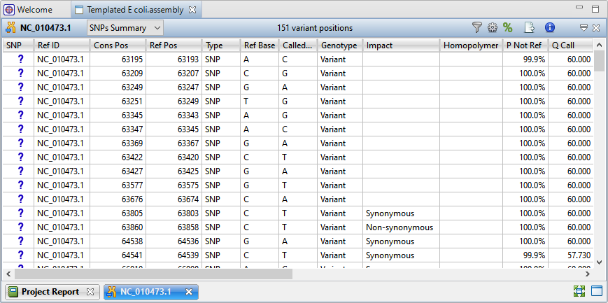
Imagine that you wish to identify those variants which are most likely to alter function of genes in E. coli. You will therefore want to focus on variations predicted to have a non-synonymous impact on the E. coli genome. In the next step, you will filter out some of the variants and only leave those predicted to cause a coding change.
- To show only variants that cause coding changes, click the Filter all variant tables tool (
![]() ) in the upper right of the view. In the Variant Filter Criteria dialog, remove the checkmarks next to Non-coding and Synonymous and click OK.
) in the upper right of the view. In the Variant Filter Criteria dialog, remove the checkmarks next to Non-coding and Synonymous and click OK.
 ) in the upper right of the view. In the Variant Filter Criteria dialog, remove the checkmarks next to Non-coding and Synonymous and click OK.
The remaining 22 variants all have a non-synonymous impact or consist of an in-frame deletion.
- Use the scrollbar on the bottom of the view to scroll right, and observe the many data columns available in this report. While each column is useful in certain circumstances, many will not be needed for this tutorial workflow.
- To remove unneeded columns from the report, click the Change alignment options tool (
![]() ). Using the image below as a guide, move all of the wanted columns “up” into the position shown below using the up arrow. Then select the remaining, unwanted, columns and press the left arrow to dismiss them. Press OK.
). Using the image below as a guide, move all of the wanted columns “up” into the position shown below using the up arrow. Then select the remaining, unwanted, columns and press the left arrow to dismiss them. Press OK.
 ). Using the image below as a guide, move all of the wanted columns “up” into the position shown below using the up arrow. Then select the remaining, unwanted, columns and press the left arrow to dismiss them. Press OK.
Note that the view is now much more compact and may be easier to view in its entirety, depending on your monitor size.
Now turn your attention to the black arrows in some of the SNP column cells. These represent “coalesced variants.” In .assembly projects like this one (but not .sqd projects), variants in adjacent columns are coalesced into a single insertion or deletion if they are of the same type, and if at least 80% of the reads with the called variant in one column have a variant in the adjacent column.
- Click any of the triangles to open the coalesced multiple-base indels and reveal individual variants. After clicking a triangle, information on each position of the insertion/deletion is displayed in a separate row.
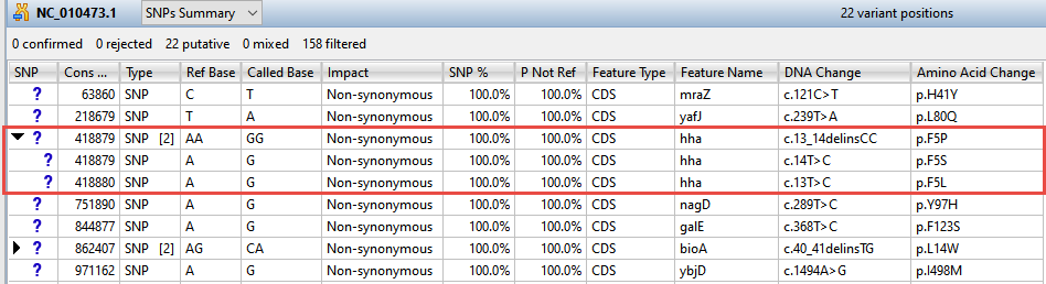
- Look at the Impact column for the variant in the first row (Cons Pos = 63860), and note that a non-synonymous mutation is predicted.
- Double-click on the row to launch the Alignment view with the variant highlighted.
The Alignment View displays the consensus sequence, and the alignment of all sequences making up a contig, at the nucleotide level. The consensus sequence for the selected contig is displayed at the top of the window, immediately beneath the ruler. Constituent sequences are displayed in the bottom section.
- Click to either side of the highlighted column to temporarily clear the selection. This will allow for a better view of the color-coding used by SeqMan Ultra.

Note that the Reference base at the position of interest is C, while all of the samples contain *T at that position. The yellow highlighting used for variants is specified in the Alignment area of the Style panel and can be changed, if desired.
- To view the variant in the Strategy view, select View > Strategy > Show Strategy View. Because two views are already open, the Strategy view appears in a pop-up window. The view graphically summarizes the position and orientation of every constituent sequence in the selected contig.
- Zoom in as far as possible by dragging the green Zoom slider (
![]() ) all the way to the right.
) all the way to the right.
 ) all the way to the right.
- Click on the top row of the Variants view table to again move the cursor to the variant of interest.
In the lower part of the window, observe the green arrows. Arrows are used to graphically represent the individual sequences in the contig. The point of the arrowhead represents the 3’ end and the tail represents the 5’ end. The green coloration of arrows in this region denotes consistent, correctly-specified paired reads.

- To add data tracks to enhance the Strategy view, click on the Tracks tab and check all boxes in the “Strategy header” section.

- Returning to the floating Strategy view window, click any plus signs appearing next to the header tracks to reveal the “hidden” tracks.
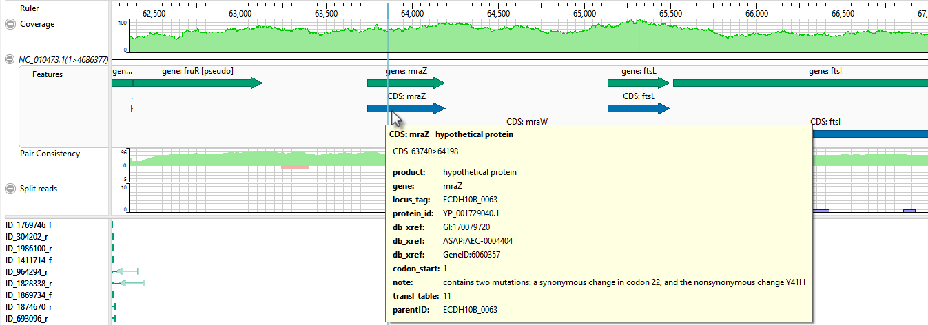
- Move the horizontal zoom slider (at the top) until you can read the feature names, as shown below. Hover over any part of a histogram to display information about that location.
![]()
- Coverage – Represents the coverage within the assembly, with green representing above-threshold coverage and red representing areas of low coverage.
- Split reads – Shows the location and depth of split reads.
- Features – The putative variant is located within a labeled CDS called mraZ.
- Pair Consistency – Shows consistent reads in green and inconsistent in red. The deeper the histogram , the more recognized pairs of reads there are.
- Coverage – Represents the coverage within the assembly, with green representing above-threshold coverage and red representing areas of low coverage.
- Close the floating Strategy view window by clicking the ‘x’ in the top corner. Then direct your view to the Variants view at the bottom of the main window.
- Confirm the variant that you just investigated by clicking on the SNP (leftmost) column to change the question mark to a checkmark. (If you had found supporting evidence was lacking, you could have clicked a second time to reject the variant and add an ‘x’.)
Short indels are included in the Variants view. However, any indels long enough to inhibit assembly are instead gathered in another report called the Structural Variation Report.
- To see the longer indels, choose Contig > NC_010473.1 Structural Variation. Scroll down to the putative Indel at 3211929.
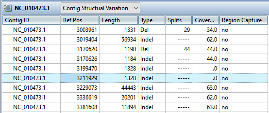
- Double-click on that table row to select it and center the Alignment view on that position. Use the horizontal zoom slider and vertical scrollbar and note that this area is devoid of reads.

This marks the end of this tutorial.
Need more help with this?
Contact DNASTAR