
- To make it easier to locate potential genes, click the object selector tool (
![]() ). Drag and drop the method names so they appear in the Legend Curtain in the order shown.
). Drag and drop the method names so they appear in the Legend Curtain in the order shown.
 ). Drag and drop the method names so they appear in the Legend Curtain in the order shown.
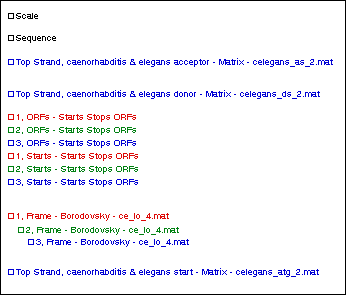
- Continuing to use the object selector, select each matrix pattern result in turn, then use Options > Line Color to change the color of the lines. For example, choose green for the donor sites, blue for the acceptor sites, and black for the start sites.
- Use the scroll bar at the bottom of the window to locate the area of the sequence around 10,000 bp.
- Select a zoom tool (
![]() ) or (
) or (![]() ) and then click on the document to enlarge or reduce the view until you can see the entire sequence range from 9,000-12,000 bp. Alternatively, select a zoom tool and then “grab” a rectangular area of the document with your mouse to zoom in on that particular region.
) and then click on the document to enlarge or reduce the view until you can see the entire sequence range from 9,000-12,000 bp. Alternatively, select a zoom tool and then “grab” a rectangular area of the document with your mouse to zoom in on that particular region.
 ) or (
 ) and then click on the document to enlarge or reduce the view until you can see the entire sequence range from 9,000-12,000 bp. Alternatively, select a zoom tool and then “grab” a rectangular area of the document with your mouse to zoom in on that particular region.
- Click the range selector tool (
![]() ) and then click on the frame 3 ORF centered on base 10,000. Note that a large peak in the frame 3 Borodovsky graph lies entirely within this highlighted ORF. It is likely that this area represents an exon.
) and then click on the frame 3 ORF centered on base 10,000. Note that a large peak in the frame 3 Borodovsky graph lies entirely within this highlighted ORF. It is likely that this area represents an exon.
 ) and then click on the frame 3
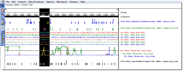
You are now ready to find the beginning of the potential gene.
- Click the object selector tool (
![]() ). In the Top Strand…atg_2.mat display, click and hold on the candidate start site at the left end of the ORF. The header shows the position of the candidate, while the pop-up information box shows the score.
). In the Top Strand…atg_2.mat display, click and hold on the candidate start site at the left end of the ORF. The header shows the position of the candidate, while the pop-up information box shows the score.
![]()
If this is the first exon of a multi-exon gene, it must end with a donor splice site that precedes the stop codon for the ORF in the same frame. In the Top Strand…ds_2.mat display, observe that there are two candidate donor splice sites (shown circled in the following figure) beyond the Borodovsky peak and still within the corresponding frame 3 ORF.
![]()
- Exon 1 Donor: Base 10028; score = 4.6
- Exon 1 Donor: Base 10056; score = 9.6
- Exon 1 Donor: Base 10028; score = 4.6

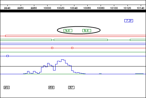
You are now ready to annotate the first exon. The position 10056 indicates the beginning of the donor splice site; therefore, the actual range of the exon extends from 9,939 to 10,055.
- Select Edit > Go to Location. Enter the range 9939,10055 and then click OK.
- Click the Annotation tool (
![]() ) to open the Feature Editor. The location of the gene segment appears in the Segment box.
) to open the Feature Editor. The location of the gene segment appears in the Segment box.
![]()
- Enter genE into the Title box.
- Enter exon1 into the Segment Name box, then click OK. A new feature is created and displayed on the Assay Document.
- Enter genE into the Title box.
 ) to open the Feature Editor. The location of the gene segment appears in the Segment box.
- Now that the first exon has been annotated, you may continue searching for additional exons. Any further exons must begin with an acceptor splice site, and that site should be in an ORF for which there is Borodovsky evidence for coding potential. Observe that the next significant Borodovsky peak is in frame 2, centered near base 10,600. There is one very likely acceptor candidate in the Top strand…as_2.mat display, between bases 10,207 and 10,219: Exon 2 Acceptor: Base 10,217; score = 12.0. If there are more than two exons to this gene, Exon 2 must terminate with a donor splice site. There is a strong candidate in the Top strand…ds_2.mat display at position 10,778, some distance to the right of where the frame-2 Borodovsky peaks fall to the baseline: Exon 2 Donor: Base 10,778; score = 12.6.
Now you may annotate this exon and join it to the first gene segment.
- Select Edit > Go to Location.
- Enter the range 10217,10777 and then click OK.
- Click the joining tool (
![]() ).
).
 ).
).- Select genE – misc_feature from the list and then click Join. The next Borodovsky peak is not only in the same frame as exon 2, but also in the same ORF. The best candidate acceptor splice site to start exon 3 has a likelihood value of 14.1 out of a maximum 16.7—an excellent candidate. Two candidate donor splice sites are available to define the 3′ end of this exon, at 10,973 and 10,993. The first site scores higher at 6.4.
- Exon 3 Acceptor: Base 10,826; score = 14.1
- Exon 3 Donor: Base 10,973; score = 6.4
- Exon 3 Acceptor: Base 10,826; score = 14.1
The next Borodovsky peak is once more in frame 2, but there is no candidate acceptor site (at the default threshold) under this peak. However, there is a site to the left of the peak, at position 11,021, that scores an impressive 15.1; this is the best candidate start for exon 4. You will note that there is no candidate donor splice site within the corresponding frame 2 ORF. This indicates that Exon 4 is probably the final exon in the gene.
To locate the stop codon:
- Select Analysis > Show Available Methods and expand Coding Prediction – Start Stops ORFs by clicking on the plus sign (Win ) or the triangle (Mac) next to the method name.
- Select the Stops method for frame 2 and drag and drop it onto the Assay Document. Notice that there is a stop codon at the end of this ORF (base 11,155). Therefore, use the splice site at base 11,021 to start this exon and the stop codon at base 11,155 to terminate this exon.
- Exon 4 Acceptor: Base 11,021; score = 15.1
- Exon 4 Donor: No likely candidates
- Stop Codon: Base 11,155
- Exon 4 Acceptor: Base 11,021; score = 15.1
- After locating the endpoints for Exons 3 and 4, annotate them by repeating steps 11-14 for each exon and entering the appropriate ranges.
- Now that all four gene segments have been annotated, click on either the object selector (
![]() ) or range selector (
) or range selector (![]() ) and then double-click on the feature to reopen the Feature Editor.
) and then double-click on the feature to reopen the Feature Editor.
- In turn, click on the coordinates for the three unnamed segments and type their names into the empty Segment Name boxes as exon2, exon3, and exon4.
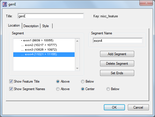
- Click OK to finish. The feature should resemble the figure below:

Proceed to Part C: Corroborate predictions via a BLAST search.
Need more help with this?
Contact DNASTAR